How to find duplicate value in Google Sheets

How to highlight cell if value duplicate in same column for google spreadsheet?

Step - 01: Select the whole column (your desired column)

Figure 01 : Google Sheets Conditional formatting

Figure 02 : Google Sheets Conditional formatting

Figure 03 : Google Sheets Conditional formatting

Figure 04 : Google Sheets Conditional formatting

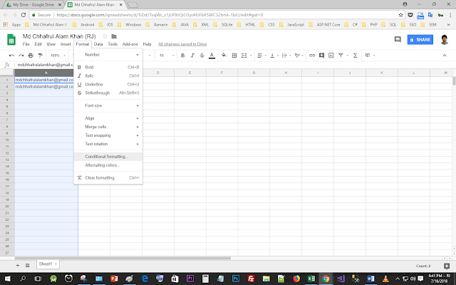
Step - 02: Click on Format menu

Figure 05 : Google Sheets Conditional formatting

Step - 03: Click Conditional formatting sub-menu

Figure 06 : Google Sheets Conditional formatting

Step - 04: Click on Format cells if... dropdown button

Figure 07 : Google Sheets Conditional formatting

Figure 08 : Google Sheets Conditional formatting

Figure 09 : Google Sheets Conditional formatting

Figure 10 : Google Sheets Conditional formatting

Step - 05: Click on Custom formula is

Figure 11 : Google Sheets Conditional formatting

Figure 12 : Google Sheets Conditional formatting

Figure 13 : Google Sheets Conditional formatting

Step - 06: Click on Value or formula text box

Figure 14 : Google Sheets Conditional formatting

Figure 15 : Google Sheets Conditional formatting

Step - 07: Type this =countif(A:A,A1)>1 formula in the Value or formula text box

Figure 16 : Google Sheets Conditional formatting

Figure 17 : Google Sheets Conditional formatting

Step - 08: Click on Formatting style dropdown button or leave it Default

Figure 18 : Google Sheets Conditional formatting

Figure 19 : Google Sheets Conditional formatting

Step - 09: Click on Fill Color icon

Figure 20 : Google Sheets Conditional formatting

Figure 21 : Google Sheets Conditional formatting

Figure 22 : Google Sheets Conditional formatting

Step - 10: Click on your desired color for highlight duplicate value in your sheets

Figure 23 : Google Sheets Conditional formatting

Figure 24 : Google Sheets Conditional formatting

Figure 25 : Google Sheets Conditional formatting

Figure 26 : Google Sheets Conditional formatting

Figure 27 : Google Sheets Conditional formatting

Step - 11: Now Click on Done button.

Figure 28 : Google Sheets Conditional formatting

Figure 29 : Google Sheets Conditional formatting

Figure 30 : Google Sheets Conditional formatting

Figure 31 : Google Sheets Conditional formatting

Figure 32 : Google Sheets Conditional formatting

Figure 33 : Google Sheets Conditional formatting

[N. B.: Ensure the range applies to your column e.g. A1:A100.
Now anything you write in the A1:A100 cells will be checked and if there is found any duplicate value then it will be coloured. For multiple columns, use countifs.]

I hope this article will help you in your work.
Thank you!